GSM receiver blocks: least squares channel estimation

I had a pretty good math tutoring session today; we looked at the least squares channel estimation problem and got it working for a simple hardcoded channel, without a transmit filter, and without upconversion/downconversion. I learned how to make a Toeplitz matrix that represents the convolution (modulated training sequence convolved against the dispersive channel) I want.

It’s a bit counter-intuitive – I’m used to thinking in terms of a vector signal being convolved by a matrix channel – but convolution commutes, so I put the signal I know (the known preamble / training sequence) into the matrix, and then do the least squares estimation by taking the pseudoinverse of that. The dimensions and contents of this matrix were unintuitive to me at first, but going over it with my tutor helped clarify it, and I’m going to explain it below.

Our channel is \(L\) (8 for GSM, which I’m using as a guide here) symbol intervals long, and the full training sequence is \(M\) (26 for GSM) symbol intervals. If there is enough radio silence before and after the training sequence is sent, we will be convolving an \(M\)-long modulated symbol vector with an \(L\)-long channel impulse response vector – in order to get an \(M+L-1\)-long received signal vector. If we’re putting the transmitted symbols inside the convolution matrix, that matrix would have to have \(M+L-1\) rows and \(L\) columns to make the dimensions match; multiply it by the channel impulse response (\(L\)-long) and get \(M+L-1\) received samples out.

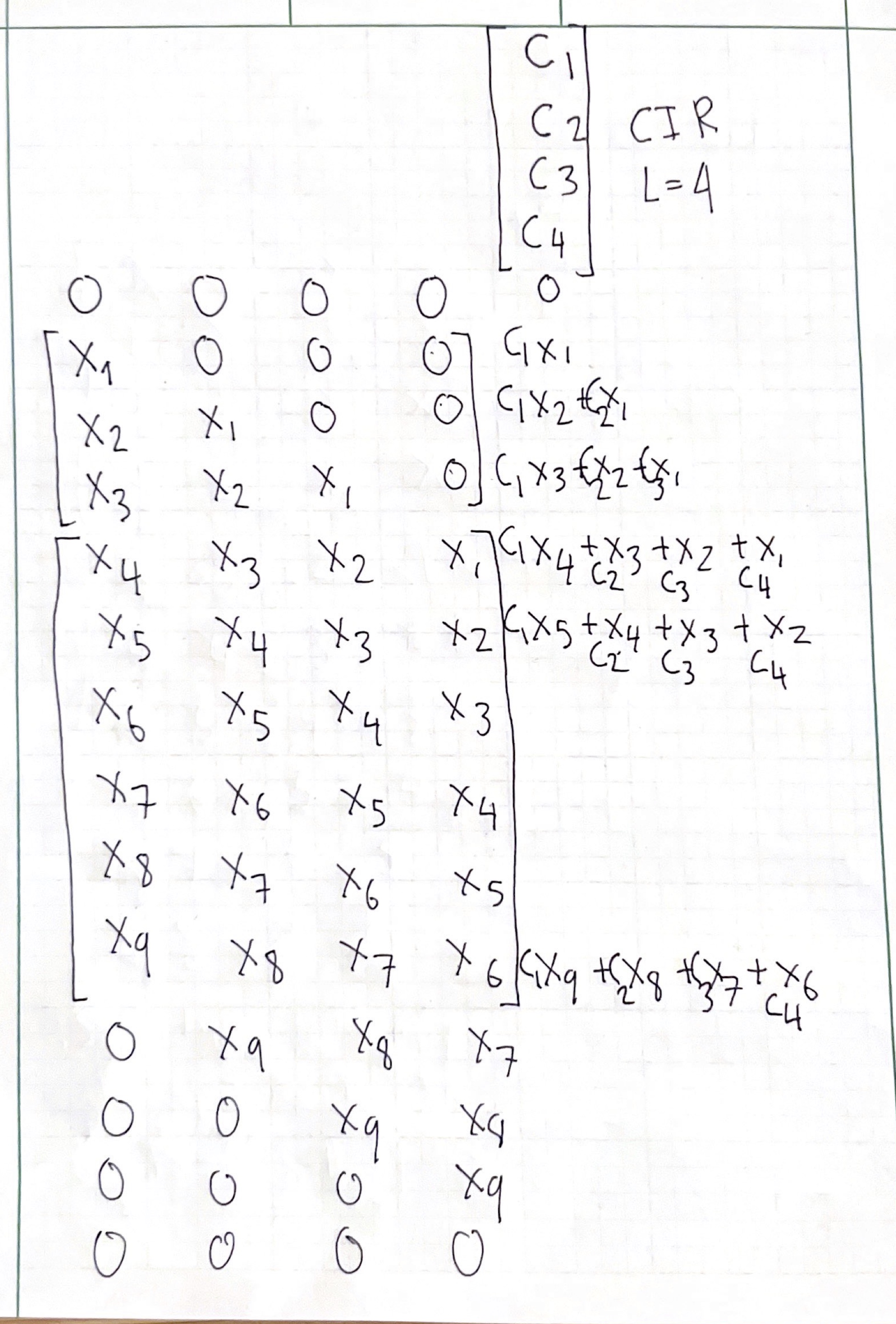
Here’s a visualisation of how the matrix multiplication works out (I let \(L=4\) and \(M=9\) to save me writing, and I’m not going to figure out how to typeset LaTeX equations with pandoc/hakyll tonight). Yeah, I forgot the \(c_1, c_2, c_3, c_4\) channel coefficients when I was writing out the dot product results :p

The received signal at any given time is the dot product of the CIR with the corresponding row of the matrix. Before we begin transmitting, the received signal is zero. The first three sampling instants are a bit odd – we start receiving signal, but not all the channel impulse response is in play.

Only at the fourth sampling instant do we have all four channel impulse response points in play. It took \(L-1=3\) timesteps of the signal being transmitted for the channel to be “filled up”. Once the channel is “filled up”, we have \(M-L+1=6\) instants we can use (and then the training sequence ends).

Now, in GSM, there isn’t radio silence before the training sequence is sent. The training sequence lives in the middle¹ of each burst, so there are data bits before and after it. The placid zeros in the convolution aren’t placid anymore – they’re data symbols, and if we need to estimate the channel before² we can figure out the transmitted symbols, they’re unknown data symbols at that!

The simple way to cope with this is to refuse to touch the first \(L-1\) samples, and run our channel impulse response estimate over the \(M-L+1\) samples after those. In GSM, this still gives us good performance, since for \(M=26\), \(L=8\) we have 19 samples to estimate 8 channel coefficients. Note that we also can’t use the trailing (in the scan, the last 4 rows) received symbols, since those also are affected by unknown data.

Now, our convolution matrix has dimensions \(M-L+1\) by \(L\), which makes sense, the only “trustworthy” (unaffected by unknown data) symbols are \(M-L+1\) long, and we are convolving by a channel of length \(L\).

In MATLAB, we can make the appropriate Toeplitz matrix with T = toeplitz(modulated_training_sequence(8:26), flip(modulated_training_sequence(1:8)));, and we use it to estimate the channel by doing estimated_chan = lsqminnorm(T, interference_rx_downsampled(64+8:64+18+8))

Figuring out the exact offset for interference_rx_downsampled has been a bit tricky, and I haven’t yet dived into writing the right correlation to estimate the exact timing offset required.

Also, using actual channels (with MATLAB’s stdchan) has led to results that don’t seem right visually, and I’m unsure why that’s the case. My suspicion is that when I call MATLAB’s resample , something weird happens to the signal, since resample has a filter of its own, and that’s going to be incorporated into the channel impulse response as well in a way that doesn’t make sense visually. Moving forward, I will try and figure out a way to measure the accuracy of the channel impulse response by looking at the sent and received signals, rather than by eyeballing it.