GSM receiver blocks: synchronization in time (part 1: the gold standard)

So now that we have a good enough channel estimation mechanism, we need to figure out how to apply it to something that vaguely looks like a real-world problem. This means no hard coding indices! We’re not going to get away with that in the real world, unless maybe we’ve got a sync cable between the transmitter and receiver…

This means we need to handle a few things:

• Timing offsets: we don’t know exactly when the training sequence starts
• Frequency offsets: local oscillators aren’t perfect
• Phase offsets: transmitter and receiver local oscillators aren’t perfectly in phase

unfazed about the phase #

Phase offsets are the easiest to handle, since those get “baked into” the channel estimate. Adding a phase offset \(\phi_{1}\) before the channel and a phase offset \(\phi_{2}\) after the channel is equivalent to multiplying the channel estimate by a complex number with magnitude 1 and phase \(\phi_{1}+\phi_{2}\). With as \(\ast\) convolution:

\[((\phi_{1} \cdot \text{transmitted}) \ast \text{channel})\cdot \phi_{2} = \text{transmitted} \ast ([\phi_{1} + \phi_{2}] \cdot \text{channel})\]

So we don’t even need to estimate a phase offset – the channel estimation handles it.

but what about the phase noise? #

We handle phase noise with the time-honored tradition of ignoring it. Seriously though, I’m not sure how much it’s a problem. I think if we have a way to update the channel estimate as it’s being used to estimate bits (“per survivor processing”), we should be able to handle it, but I’m nowhere near that yet.

we’ll fret about the freqs later #

A frequency offset will show up as a changing phase offset, and this won’t be handled by the channel estimation – unless, again, if we have a way to update the channel estimate as it’s being used in the actual demodulation.

Fortunately, we can estimate and compensate for frequency offsets earlier in the receiver and without needing the ability to estimate/update the channel estimate. In fact, we likely can get better results by compensating for frequency error with a mechanism designed for that purpose, that can operate over the entire received burst at once.

In actual GSM, coarse frequency synchronization is handled by the “frequency burst”; which carries no data but is designed to allow easy recovery of the carrier frequency at the mobile station. We’ll look at how to handle frequency offsets in a future post.

time for timing #

Similarly, in actual GSM, coarse time synchronization is handled by the “synchronization burst” – which has an extra-long training sequence and information that identifies the base station.

We will look at how to handle time offsets in this post. The synchronization burst is a special case of a normal burst, and we can use the same methods to handle both.

let the loss be your guide #

I spent some time guessing various indices for the least squares and eyeballing “how good” (with a channel generated by conv(modulated, [1,2,3,4,5,4,3,2]); ) the channel estimate was, which was kind of elucidating but not very principled.

Fortunately, we have a better tool: the least squares loss function.

We stop using the hardcoded channel [1,2,3,4,5,4,3,2] with its mysteriously-integer-valued coefficients, and use interference_channel = stdchan("gsmEQx6", nominal_sample_rate, 0); instead, and we add some AWGN: awgned = awgn(received,10);. Here’s the code:

entire example code #

training_sequence = [0,1,0,0,0,1,1,1,1,0,1,1,0,1,0,0,0,1,0,0,0,1,1,1,1,0]';

data = [randi([0 1],64,1); training_sequence; randi([0 1], 128,1)];


modulated = minimal_modulation(data);
nominal_sample_rate = 1e6 * (13/48);

interference_channel = stdchan("gsmEQx6", nominal_sample_rate, 0);


%received =  conv(modulated, [1,2,3,4,5,4,3,2]);
%received = conv(modulated, [1,1,0,0,0,0,0,0]); 
received = interference_channel(modulated);
nominal_channel_length = 8


modulated_training_sequence = minimal_modulation(training_sequence);
training_sequence_length = length(training_sequence)


toeplitz_column = modulated_training_sequence(nominal_channel_length:training_sequence_length);
toeplitz_row = flip(modulated_training_sequence(1:nominal_channel_length));
T = toeplitz(toeplitz_column, toeplitz_row);

awgned = received % awgn(received,10);

clean_part_of_training_sequence = training_sequence_length - nominal_channel_length;

losses = ones(1, length(received)-clean_part_of_training_sequence);

for offset = 1:(length(received)-clean_part_of_training_sequence)

	interesting_part_of_received_signal = awgned(offset:offset+clean_part_of_training_sequence);
	estimated_chan = lsqminnorm(T, interesting_part_of_received_signal)

	loss_vector = T* estimated_chan - interesting_part_of_received_signal;
	TS_losses(offset) = norm(loss_vector);
end

[val, best_offset] = min(TS_losses);

interesting_part_of_received_signal = awgned(offset:offset+clean_part_of_training_sequence);
best_estimated_chan = lsqminnorm(T, interesting_part_of_received_signal)


function not_really_filtered = minimal_modulation(data) 
	not_really_filtered = pammod(data,2);
end

brute force timing estimation #

The relevant section for what we’re doing today is below. We try every possible offset, and we see which one gives us the smallest loss:

losses = ones(1, length(received)-clean_part_of_training_sequence);

for offset = 1:(length(received)-clean_part_of_training_sequence)

	interesting_part_of_received_signal = awgned(offset:offset+clean_part_of_training_sequence);
	estimated_chan = lsqminnorm(T, interesting_part_of_received_signal)

	loss_vector = T* estimated_chan - interesting_part_of_received_signal;
	TS_losses(offset) = norm(loss_vector);
end

[val, best_offset] = min(TS_losses);

interesting_part_of_received_signal = awgned(offset:offset+clean_part_of_training_sequence);
best_estimated_chan = lsqminnorm(T, interesting_part_of_received_signal)

Yeah, we redo the least squares calculation, but it’s not a big deal. This is a terribly slow way to do timing synchronization anyway, but it’s excellent to figure out what is going on.

this is loss #

We plot(TS_losses) and get an unambigous and deep correlation dip:

Looking at how we calculated TS_losses, we see that it’s only calculated over the training sequence, not over the whole burst. We are curious to see what happens if we calculate the “error” over the whole burst. We’ll do this by convolving the transmitted signal (before the channel) with the estimated channel, and then subtracting the received signal:

>> tiledlayout(2,1)
>> nexttile
>> plot(abs(received))
>> title("actual received signal")
>> fake_received_signal = conv(best_estimated_chan, modulated);
>> nexttile
>> plot(abs(fake_received_signal))
>> title("fake received signal")
>> copygraphics(gcf)

and they don’t look very similar at all :(

Either we made a big mistake, or there’s behavior in the real channel that a convolution with the estimated channel is failing to capture.

the fake, in its attempt to be real #

We try and plot the difference, praying that there might be something interesting there…and get an error.

>> plot(abs(received-fake_received_signal))
Arrays have incompatible sizes for this operation.

This leads us to look at the sizes, and more specifically, the difference in sizes:

>> size(fake_received_signal)

ans =

   225     1

>> size(received)

ans =

   218     1

>> 218-225

ans =

    -7

7 is sus because it’s almost 8, the putative channel size in GSM. We look at the plots again, and we observe that the actual received signal is preceded by samples that look…zero-ish, and exactly 7 of them at that:

>> received

received =

  -0.0000 + 0.0001i % 1
  -0.0014 - 0.0006i % 2
   0.0027 + 0.0010i % 3
  -0.0003 - 0.0022i % 4
   0.0019 + 0.0056i % 5
  -0.0040 - 0.0044i % 6
   0.0018 + 0.0033i % 7
   0.1531 + 0.2801i
   0.2313 + 0.2729i
   0.3761 - 0.1057i
  -0.1923 - 0.1956i
  -0.7524 - 0.6256i

This hasn’t had AWGN added – this is just from the effect of stdchan("gsmEQx6", nominal_sample_rate, 0). It looks like this Matlab channel simulation is flushing the channel with some noise, since the modulated signal doesn’t look like this at all:

>> modulated

modulated =

   1.0000 + 0.0000i
   1.0000 + 0.0000i
  -1.0000 + 0.0000i
  -1.0000 + 0.0000i
  -1.0000 + 0.0000i
   1.0000 + 0.0000i
  -1.0000 + 0.0000i
  -1.0000 + 0.0000i
   1.0000 + 0.0000i
   1.0000 + 0.0000i

If we run a cross-correlation between this “fake” received signal (generated by convolving the original modulated signal with the estimated channel) and the actual received signal, we get something remarkably disappointing:

>> fake_received_signal = conv(best_estimated_chan, modulated);
>> [c, lagz] = xcorr(received, fake_received_signal);
>> stem(lagz,abs(c))

If we zoom in on the center, we see it’s unfortunately nowhere near sharp:

It’s still unclear exactly what is going on – the behavior differences at the beginning/end of the channel simulation fail to explain the catastrophic lack of similarity.

return to a simpler channel #

We go back to our contrived, integer-valued channel:

received =  conv(modulated, [1,2,3,4,5,4,3,2]);

and run this again. To make things really simple, we turn off the noise:

awgned = received;

We plot TS_loss and see a perfect zero loss at an offset of 72 (64 + 8):

but the best estimated channel is nowhere near the actual channel, which is [1,2,3,4,5,4,3,2]:

>> best_estimated_chan

best_estimated_chan =

    1.2873
    0.3579
   -1.0171
   -0.6468
   -0.5164
   -0.3579
   -3.1032
   -2.9164

>> 

it’s a bug #

So we take a look at our code again, and we find a plain old bug:

for offset = 1:(length(received)-clean_part_of_training_sequence)

	interesting_part_of_received_signal = awgned(offset:offset+clean_part_of_training_sequence);
	estimated_chan = lsqminnorm(T, interesting_part_of_received_signal)

	loss_vector = T* estimated_chan - interesting_part_of_received_signal;
	TS_losses(offset) = norm(loss_vector);
end

[val, best_offset] = min(TS_losses)

interesting_part_of_received_signal = awgned(offset:offset+clean_part_of_training_sequence);
best_estimated_chan = lsqminnorm(T, interesting_part_of_received_signal)

In the penultimate line, where we slice out the part of the received signal we’ll run a least-squares on, the indices for the slice are(offset:offset+clean_part_of_training_sequence).

offset is the loop variable, and its value there is quite simply the offset of the last least-squares computed in the loop. It is not best_offset, which is the index of the minimum loss.

We fix this, and now the best estimated channel is indeed what we expect it to be:

best_estimated_chan =

    1.0000
    2.0000
    3.0000
    4.0000
    5.0000
    4.0000
    3.0000
    2.0000

a brief detour in shoggoth-land #

Out of curiosity, I gave the above excerpt to ChatGPT-4 preceded by the prompt “find the bug:”, and it figures it out perfectly!

GPT-3.5 didn’t clue in on it, and even GPT-4 didn’t clue in on it when fed the whole file’s contents rather than the excerpt.

validating the fix #

With this fix in place, we see that the fake received signal (generated by convolving the transmitted signal with the best estimated channel) is indeed identical to the original received signal, at least with the contrived channel:

looking at real channels again #

We go back to the real channel (well, it’s not an actual IRL channel but it’s a simulation of an IRL channel), and see how much better our “fake” (generated by convolving the transmitted signal with the best estimated channel) received signal is:

Now this is a specimen!

This is, effectively, the same signal, except for subtleties in how the beginning and end are handled. It looks like the channel simulator flushes (seasons?) the beginning of the channel with very low-amplitude noise, and handles the end by “cutting off” the simulation before letting the channel “drain”, whereas the simplistic convolution doesn’t prepend low-amplitude noise at the beginning and lets the channel completely drain out.

If we add sufficient zeros to the beginning and end of the modulated signal, and feed it in both the channel simulation and the convolution:

>> received = interference_channel([zeros(16,1);modulated;zeros(16,1)]);
>> tiledlayout(2,1)
>> nexttile
>> plot(abs(received))
>> title("actual received signal")
>> fake_received_signal = conv(best_estimated_chan, [zeros(16,1);modulated;zeros(16,1)]);
>> nexttile
>> plot(abs(fake_received_signal))
>> title("fake received signal")
>> copygraphics(gcf)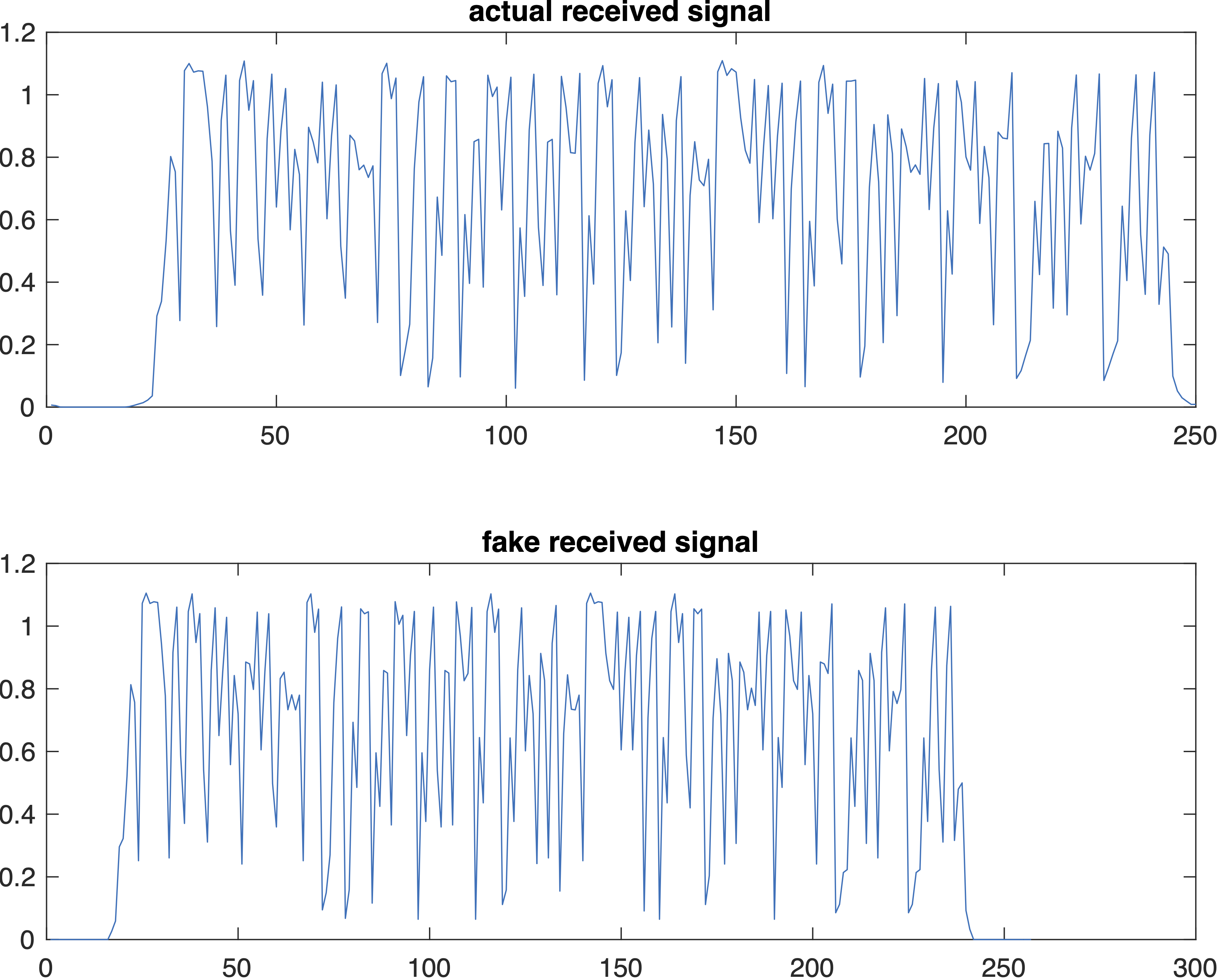

Since these are complex signals, we should be sure that the real/imaginary parts match, and not just the magnitudes:

>> received = interference_channel([zeros(16,1);modulated;zeros(16,1)]);
>> fake_received_signal = conv(best_estimated_chan, [zeros(16,1);modulated;zeros(16,1)]);
>> tiledlayout(2,2)
>> nexttile
>> plot(real(received))
>> title("received signal, real")
>> nexttile
>> plot(imag(received))
>> title("received signal, imag")
>> nexttile
>> plot(real(fake_received_signal))
>> title("fake received signal, real")
>> nexttile
>> plot(imag(fake_received_signal))
>> title("fake received signal, imag")
>> copygraphics(gcf)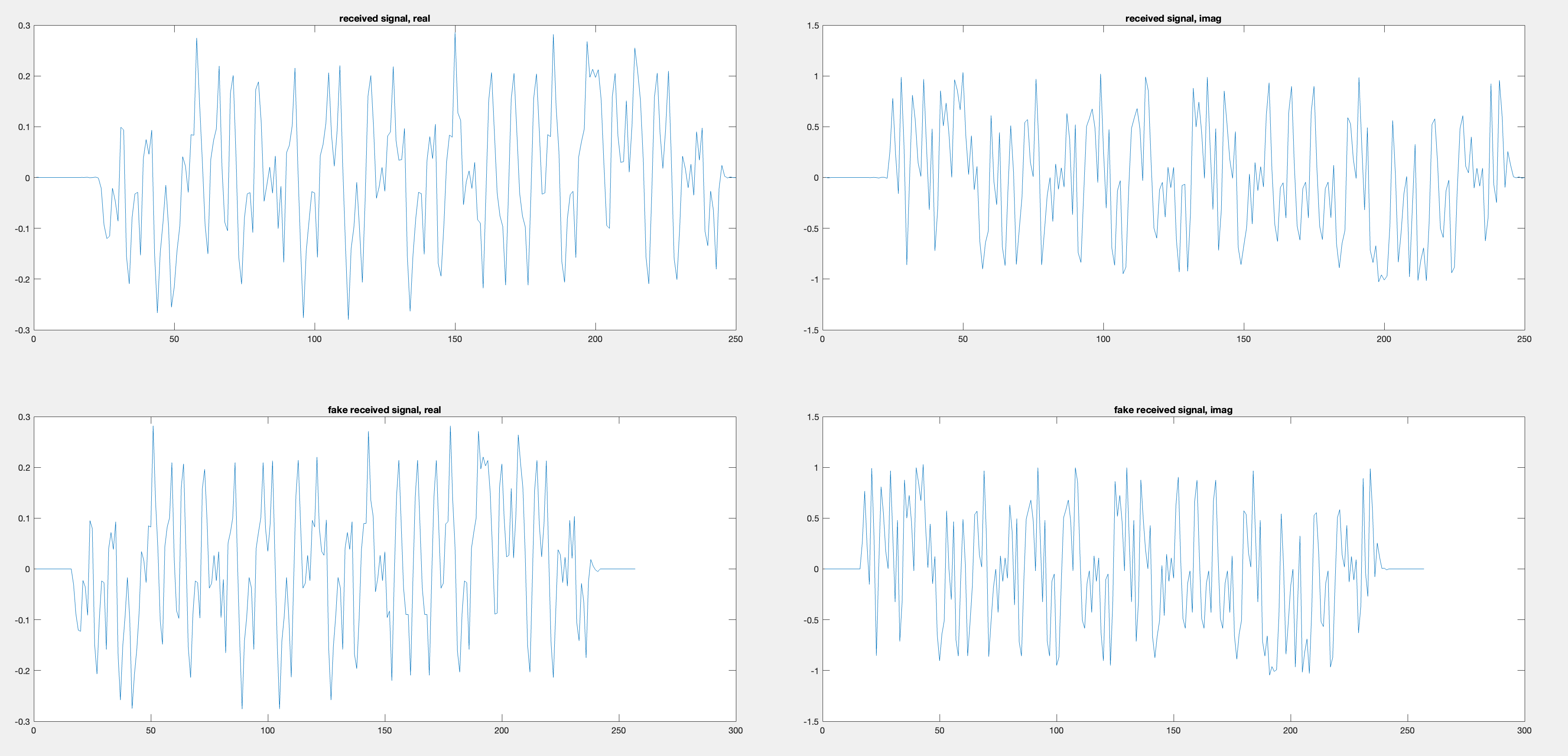

Looks good!

a simpler method will wait for next time #

We’ve actually made a working time synchronization estimator! Unfortunately it’s incredibly inefficient – requiring a whole least-squares estimate for every possible offset. However, it will serve as an ironclad gold standard¹ and help us build a more efficient synchronization estimator next time.