GSM receiver blocks: GMSK and Laurent

Not all modulation schemes have the zero-ISI property that RRC-filtered ¹ linear modulations have. Continuous-phase modulations (like GMSK, which we’ll be looking at) generally introduce inter-symbol interference: if your receiver recovers symbols by slicing-and-thresholding the received-and-filtered signal, it will have degraded performance – even if its timing is perfect.

This doesn’t prevent us from making high-performance (approaching optimal) receivers for GMSK. If the transmitter has a direct line-of-sight to the receiver and there’s not much else in the physical environment to allow for alternate paths, the channel won’t have much dispersive effect. This lets us approximate the channel as an non-frequency-selective attenuation followed by additive white Gaussian noise. In this case, you can use the Laurent decomposition of the GMSK amplitude-domain waveform to make a more complex receiver that’s quite close to optimal.

The former case is common in aerospace applications: if an airplane/satellite is transmitting a signal to an airplane/satellite or to a ground station, there usually is a quite good line of sight between the two – with not many radio-reflective objects in between that could create alternate paths. The received signal will look very much like the transmitted signal, only much weaker.

If your transmitter and receiver antennae aren’t in the sky or in space, they’re probably surrounded by objects that can reflect radio waves. In fact, they might not even have any line of sight to each other at all! You can use your cell phone anywhere with service, not just anywhere you have a cellular base station within line of sight.

If you’ve ever spoken loudly in a quiet tunnel/cave/parking garage, you hear echoes – replicas of your voice, except delayed and attenuated. A similar phenomenon occurs when there’s multiple paths the radio waves can take from the transmitter to the receiver. Think of the channel as a tapped delay line: the receiver receives multiple copies of the signal superimposed on each other, with each copy delayed by the corresponding path delay and attenuated by the corresponding path loss.

in which we ignore doppler #

Imagine an extreme case: sending symbols at \(1\) symbol per second, and leaving the channel silent for \(1\) second between each symbol. Let’s say we have four fixed paths with equal attenuation, with delays \(50\)ms, \(100\)ms, \(150\)ms, and \(210\)ms. The difference between the shortest path (the path that will start contributing its effect at the receiver the earliest) and the longest path (the path that takes the longest time to start contributing its effect at the receiver) is known as the “delay spread” and here, it’s \(210-50\)ms\(=160\)ms. Initially, receiver gets something very much non-constant: after each of the paths “get filled up”, they appear at the receiver, but only happens in the first \(160\)ms of the symbol. However, after that \(160\)ms, the channel reach equilibrium, and for the remaining \(1000\)ms\(-160\)ms\(=840\)ms, the receiver receives a constant signal. If the receiver ignores the first \(160\)ms of each symbol, it can ignore the multipath altogether!

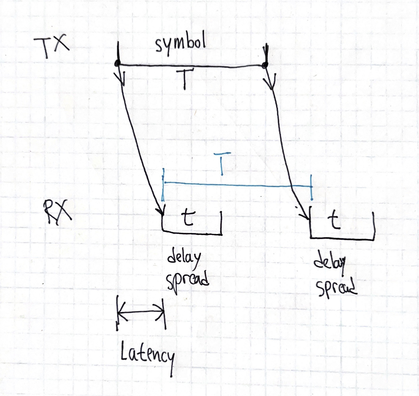
big T is the symbol length, small t is the delay spread — big \(T\) is the symbol length, small \(t\) is the delay spread

Note that the absolute delay of the paths does impacts the latency of the system, but it doesn’t impact how the channel corrupts the signal. You could imagine the same system, except that there’s 3,000,000 kilometers of ideal (doesn’t attenuate or change the signal, just delays it) coaxial cable between the transmitter and the transmit antenna. That’s gonna add 10 seconds² of delay, but it won’t alter the received signal at all.

This dynamic (symbol time much greater than delay spread) is why analog voice modulation doesn’t need fancy signal processing to cope with multipath. The limit of human hearing is 20 kilohertz, and \(c/(20kHz)=15\) kilometers, which is pretty big – paths with multiple kilometers of additional distance are gonna be pretty attenuated and won’t be very significant to the receiver³.

The higher the data rate compared to the delay spread, the less you can ignore multipath. Increase the symbol rate to GSM’s \(270\) kilosymbols per second, and we get \(c/(270kHz)=1\) kilometer. Paths with hundreds of meters of additional distance aren’t negligible in lots of circumstances!

A high-performance demodulator has to function⁴ despite this channel-induced ISI. It turns out that the same mechanism that needs to handle the channel-induced ISI (which changes based on the physical arrangement of the scatterers in the environment, and is estimated by the receiver, often using known symbols) can also handle the modulation-induced ISI as well.

the Laurent decomposition #

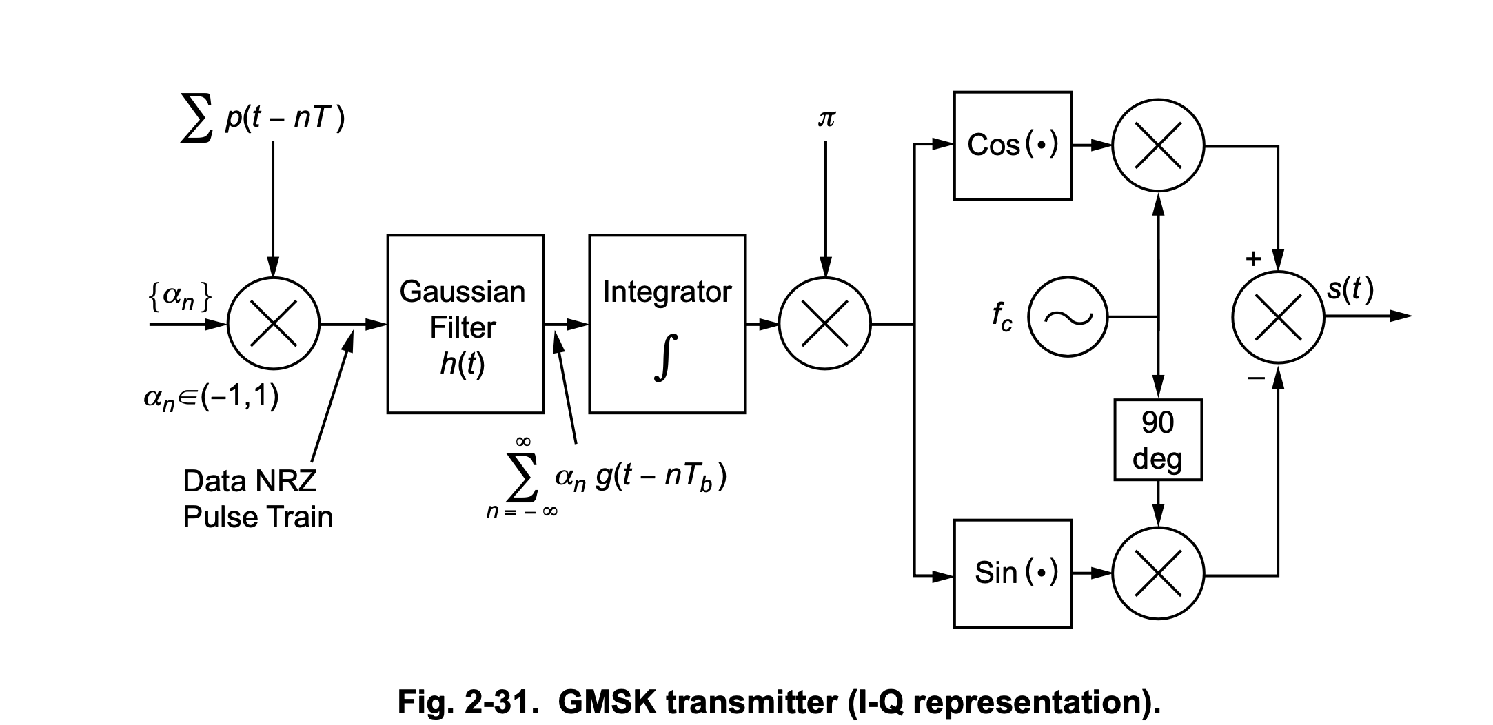
The “Gaussian” in “GMSK” isn’t a filter that gets applied to the time-domain samples. Rather, it’s a filter that gets applied in the frequency-domain, and this frequency-domain signal gets used to feed an oscillator – and it’s that oscillator that generates the time-domain baseband signal.

The following 3 diagrams are from the wonderful Chapter 2 of Volume 3 of the JPL DESCANSO Book Series.

How GMSK gets made. Source: Page 65, Chapter 2, Volume 3, JPL DESCANSO Book Series

The Laurent decomposition tells us that the Gaussian-shaped GMSK frequency-domain pulse, after it gets digested by an oscillator, ends up being equivalent to two time-domain pulses (there are more but they are truly negligible), \(C_0\) (the big one) and \(C_1\) (the small one):

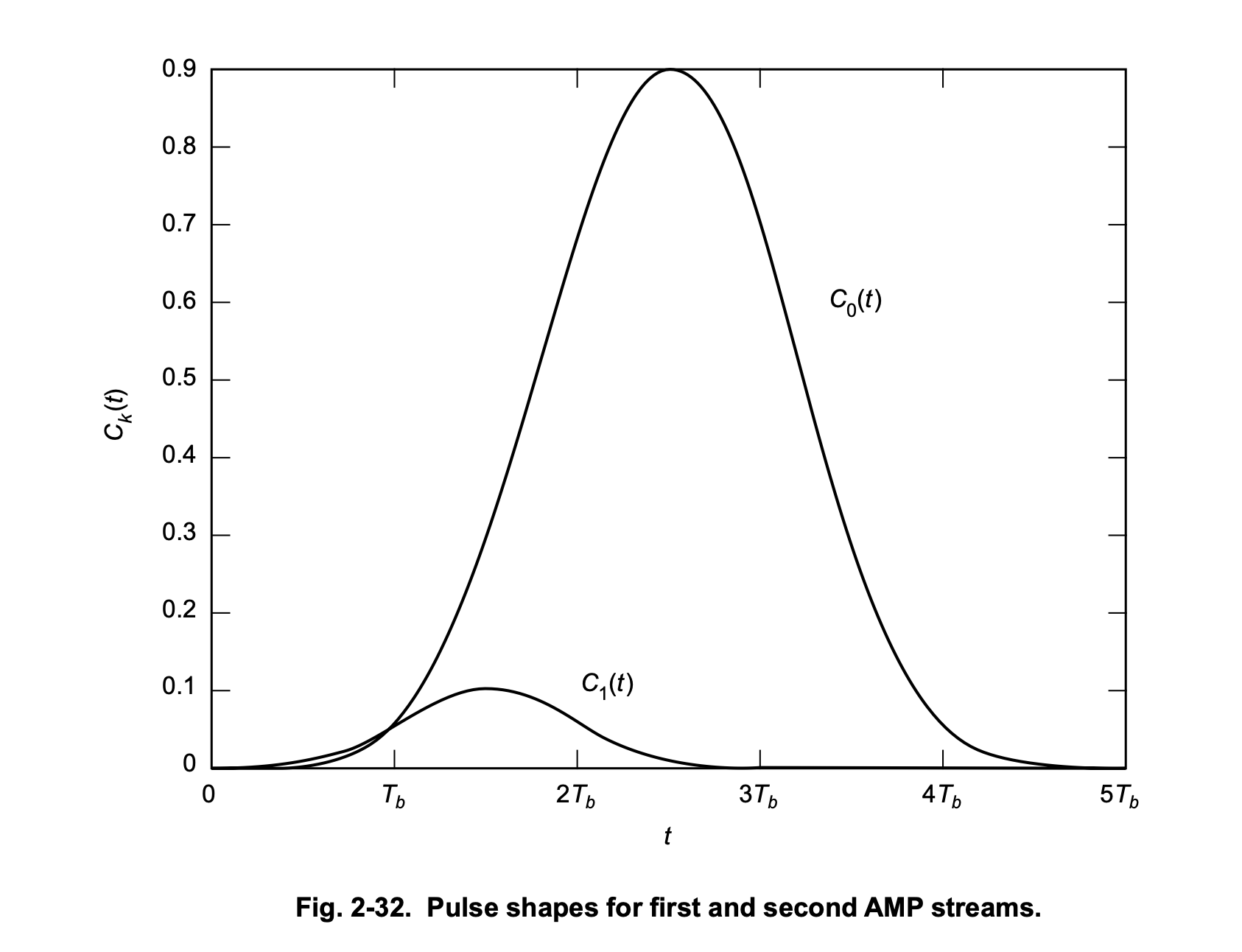
The two Laurent decomposition pulses for GMSK. Source: Page 74, Chapter 2, Volume 3, JPL DESCANSO Book Series

How to use the two Laurent pulses to produce a GMSK waveform. Source: Page 79, Chapter 2, Volume 3, JPL DESCANSO Book Series

The first Laurent pulse is excited by a function of the current data symbol⁵. So far, so good. A suboptimal receiver can pretend that a GMSK waveform is only made of \(C_0\) Laurent pulses. If you ignore the \(C_1\) pulse, this reduces GMSK to MSK. MSK is not a linear modulation, and has nonzero ISI: the amplitude-domain pulse doesn’t have the zero-ISI property that RRC has.

However, if we have a good phase estimate, we can separate the MSK signal into in-phase (\(I\)) and quadrature (\(Q\)) signals. MSK⁶ has a wonderful property once we’ve decomposed it this way: The “useful channel” alternates between \(I\) and \(Q\) for every symbol and contains no ISI, and the “other channel” (which alternates between \(Q\) and \(I\)) contains all the ISI.

To phrase it another way, on even symbols, the information needed to estimate the symbol is all in \(I\), and the ISI is all in \(Q\), and on odd symbols, the information needed to estimate the symbol is all in \(Q\), and the ISI is all in \(I\). Looking at \(I\) and \(Q\) separately eliminates the ISI, and this lets us make a receiver that looks much like a linear modulation receiver (integrate-and-dumps, comparators, etc) with close to ideal performance.

the modulator has memory #

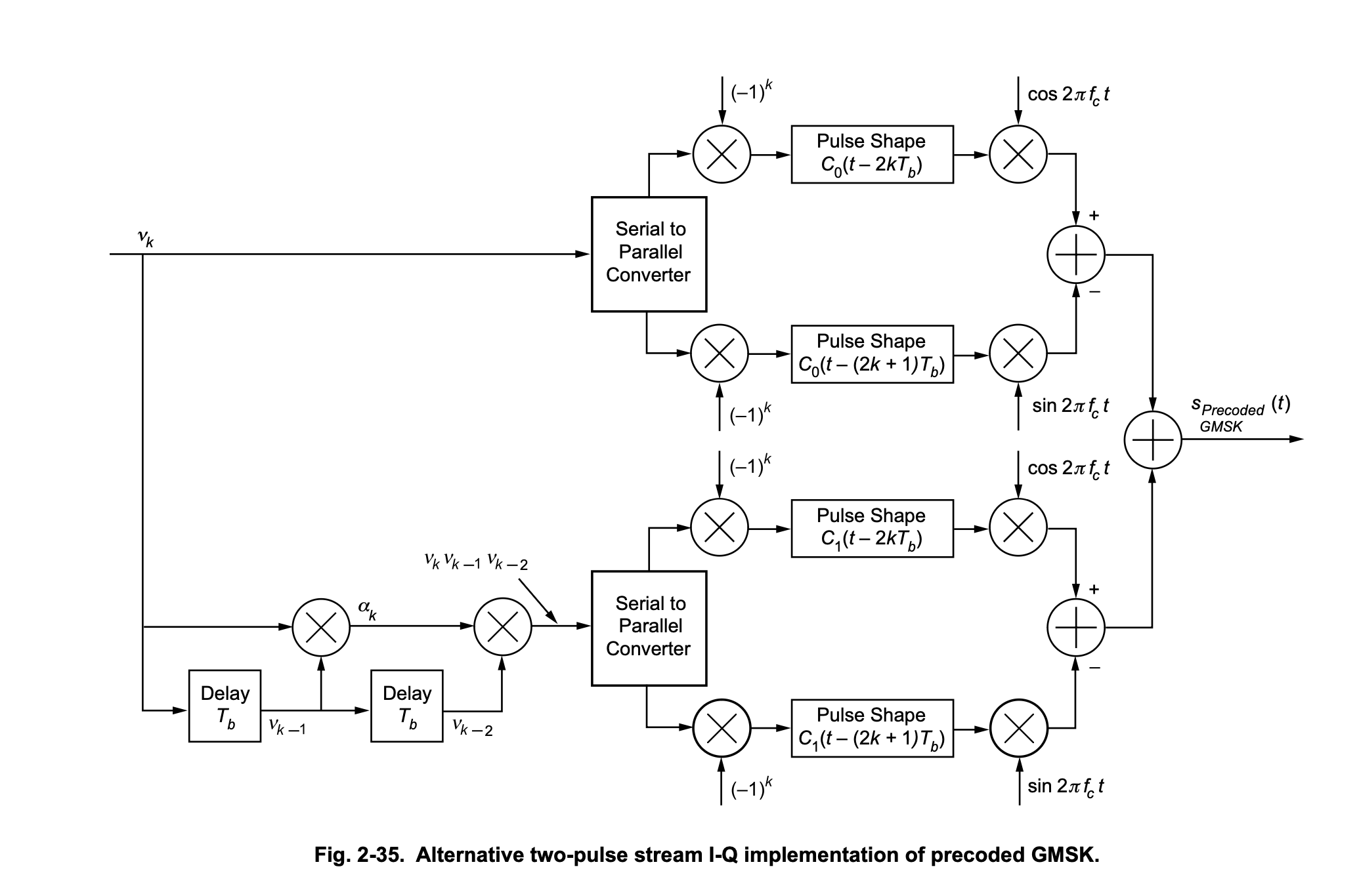
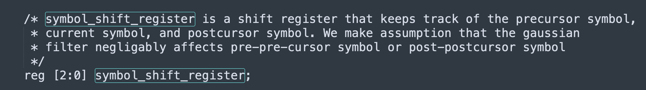
Stuff gets more interesting if you don’t ignore the second Laurent pulse. What’s that one excited by? Well, it’s a function of the current bit, the previous bit, and the bit before that! There’s even a little shift register on the bottom left!

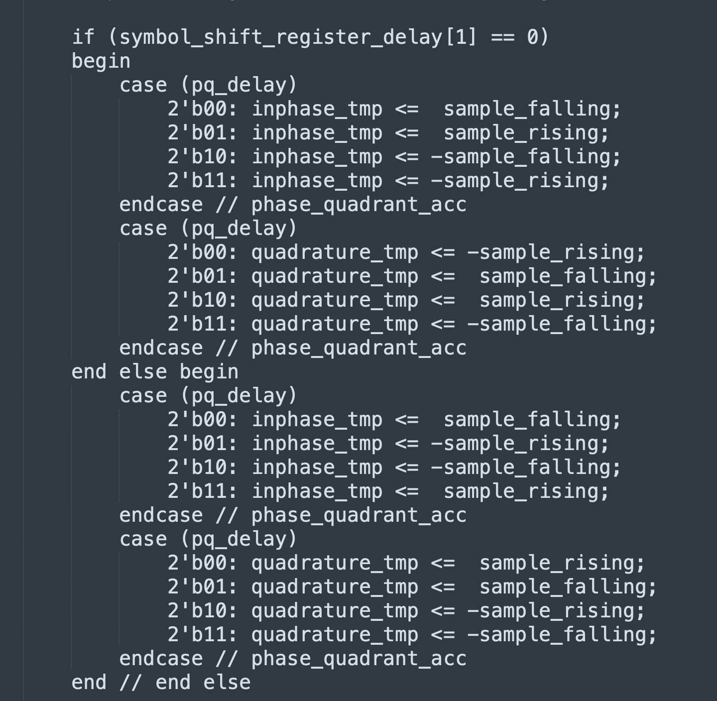
Incidentally, that shift register isn’t just theoretical. If you implement a GMSK modulator with precomputed waveforms in a ROM (as opposed to using a Gaussian filter / integrator / NCO), there’s gonna be a shift register that looks much like that, which helps you index the ROM and postprocess the ROM output. I implemented a GMSK modulator in Verilog that uses precomputed waveforms, with the paper “Efficient implementation of an I-Q GMSK modulator” (doi://10.1109/82.481470 by Alfredo Linz and Alan Hendrickson) as a guide.

GMSK modulator architecture. Source: Linz1996 (doi://10.1109/82.481470)

I define that shift register in my Verilog. Source: a GMSK modulator I wrote a while ago, based on the design in Linz1996 (doi://10.1109/82.481470)

Shifting in new data symbols into the shift register. Source: a GMSK modulator I wrote a while ago, based on the design in Linz1996 (doi://10.1109/82.481470)

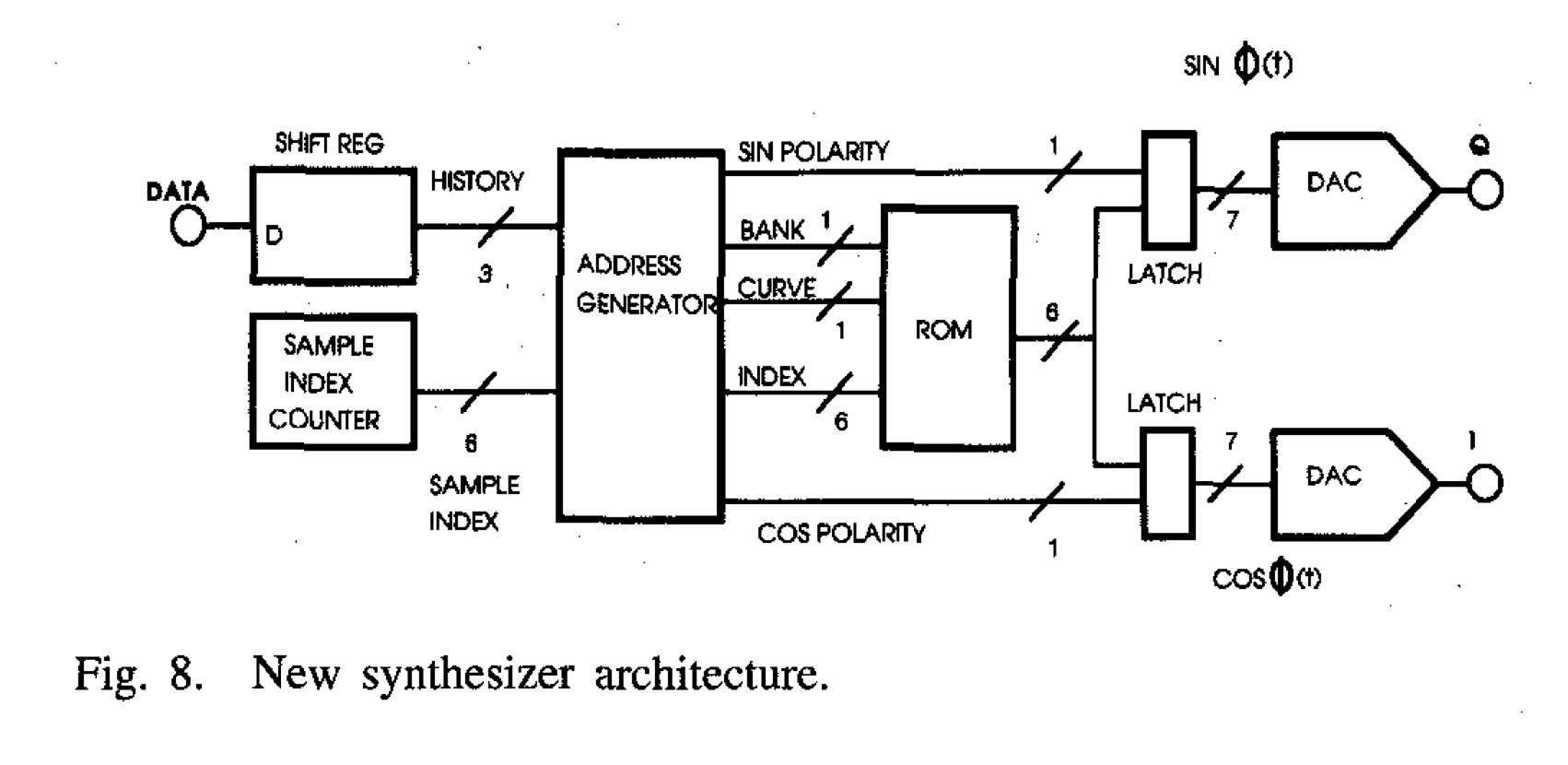
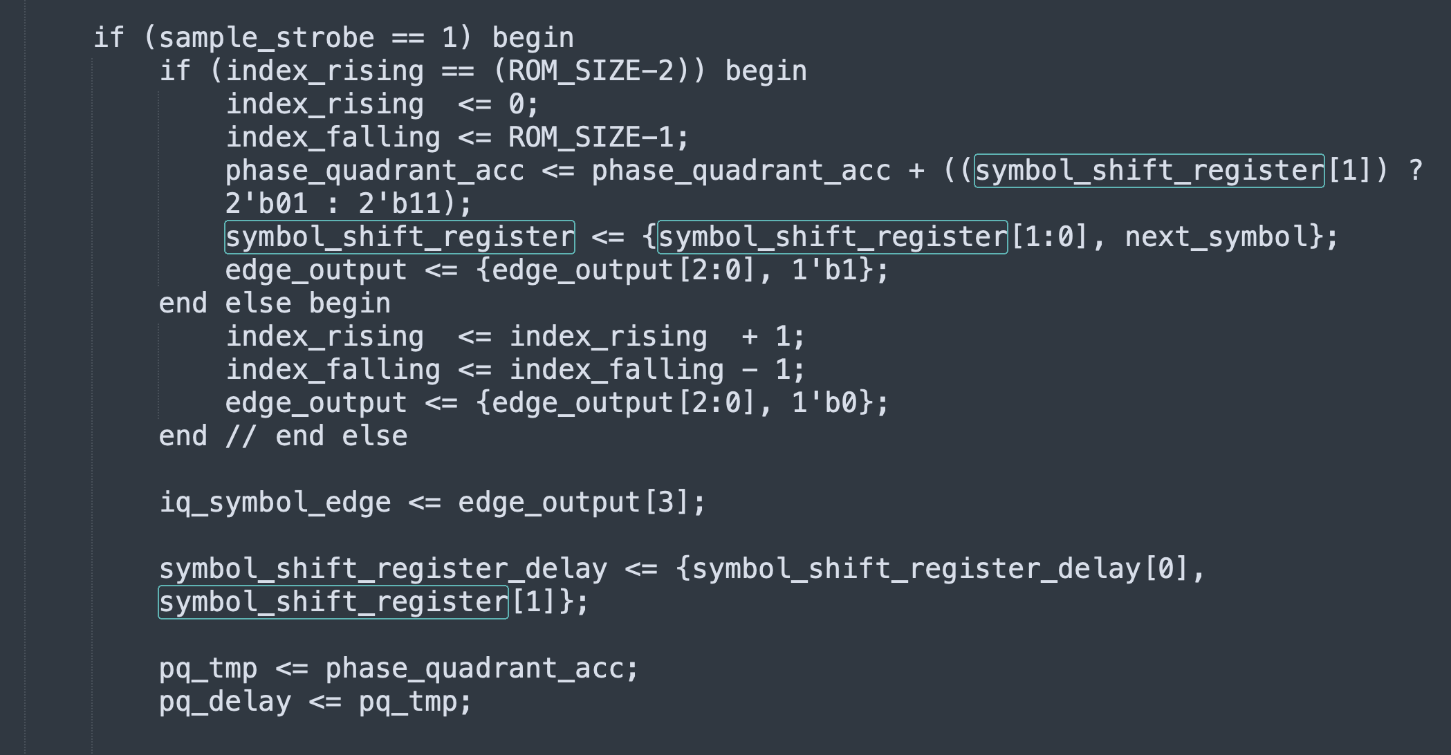
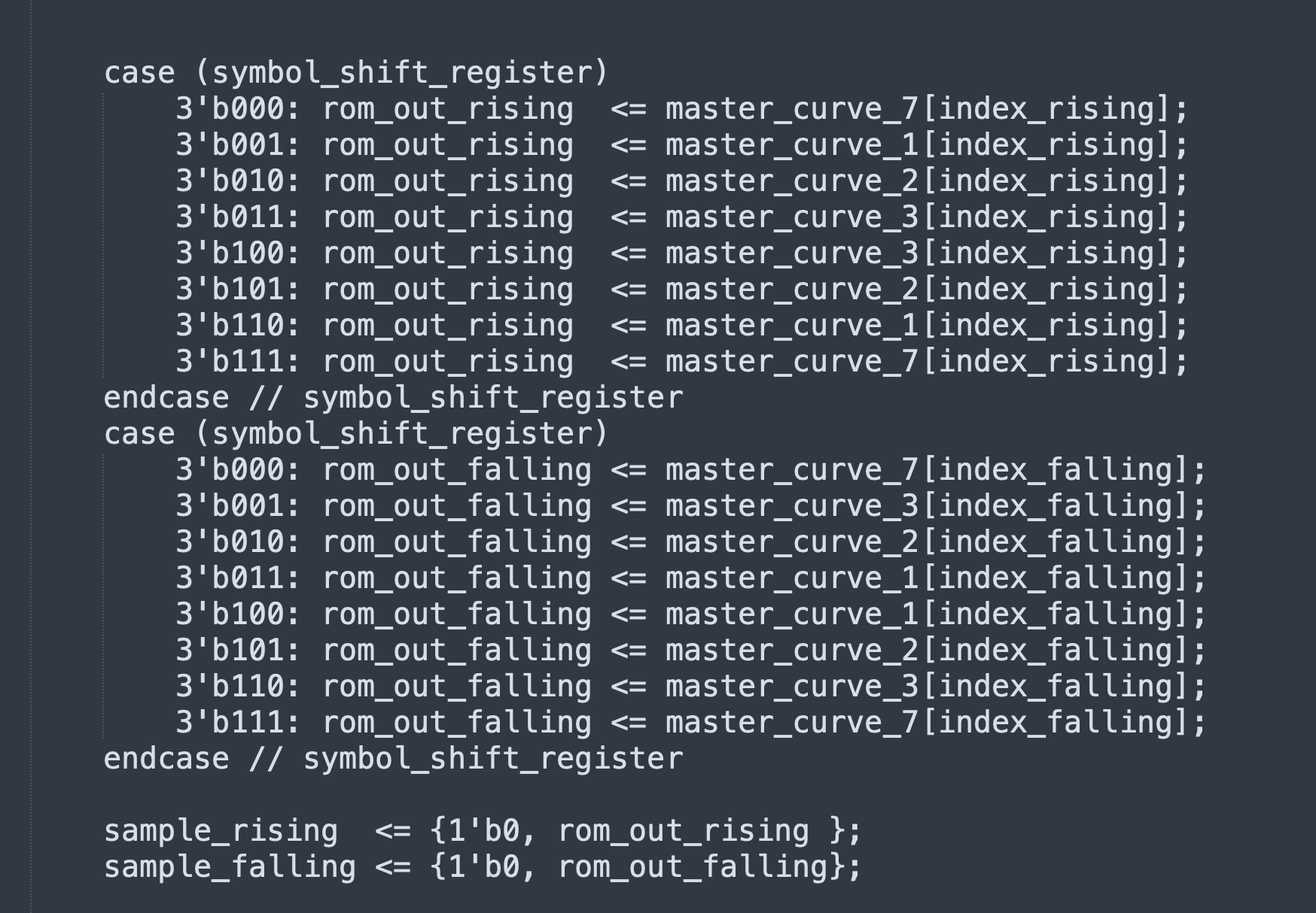
There’s 16 possible waveforms you need to be able to generate (8 possible values of the shift register; I and Q for each), but the structure of the modulation lets you cut down on ROM required: if you can time-reverse (index the ROM backwards) and/or sign-reverse (flip the sign of the samples coming out of the ROM), you can store just 4 basic curves in the ROM and generate all 16 waveforms that way.

The shift register determines which basic curves get used. Source: a GMSK modulator I wrote a while ago, based on the design in Linz1996 (doi://10.1109/82.481470)

One bit of the shift register, along with another bit of state (accumulated phase quadrant), determines how we post-process the output of the ROM. Source: a GMSK modulator I wrote a while ago, based on the design in Linz1996 (doi://10.1109/82.481470)

Unlike with RRC, there’s no magic filter that nulls out GMSK’s ISI/memory. Unlike with MSK, separating \(I\) and \(Q\) doesn’t neatly separate the data and the ISI.

detection theory tl;dr #

Every time a demodulator receives a new sample (or receives \(n\) new samples if there are \(n\) samples per symbol), it needs to decide what symbol was most likely to generate that sample. If it didn’t do something like that, it wouldn’t be much of a demodulator.

If the modulator has no memory, this task is pretty simple: we look at the sample values each possible symbol would have generated, and we compare each of those gold-standard values against the value we actually received. Which symbol was most likely to have been sent? The symbol whose value is the closest to what was actually received.

How accurate is this? Depends on how many possible symbols there are! Increase the number of possible symbols (“bits per symbol”, “modulation order”), and this decreases the amplitude of noise necessary to sufficiently shift the received sample such that the closest symbol is incorrect.

the third eye of the demodulator #

If the modulator has memory, this task is more complicated. The signal that the modulator generates for a symbol don’t just depend on the current symbol, but on a certain number of past symbols as well.

If the demodulator wants to extract the most possible information from the received signal, it needs to read the modulator’s mind.

Assume the demodulator has access to a perfect mind-reading channel: we can see into all of the modulator’s state – except for what’s affected by the current symbol. The latter proviso prevents the demodulator’s task from becoming trivial. Via the mind-reading channel, the demodulator knows the last two bits the modulator sent: call them \(b_1\) and \(b_2\). There’s a standard assumption that the transmitted signal is a random bitstream, so knowing \(b_1\) and \(b_2\) gives the demodulator strictly zero information about \(b_3\).

The demodulator actually has to estimate \(b_3\) from the noisy received signal, like usual. However, that task is actually solvable now! We have a local copy of a GMSK modulator, and we generate two candidate signals: one with the sequence \((b_1, b_2, 0)\), and one with the sequence \((b_1, b_2, 1)\). If what was actually received is closer to the former, we decide a \(0\) was sent, if the latter is closer, we decide a \(1\) was sent.

You see where this is going! We estimated a value for \(b_3\) – call it \({b\_estimated}_3\) – by comparing the two possible alternatives. Now, when the modulator sends \(b_4\), we don’t need the mind-reading channel anymore! We already have our best estimate for what \(b_3\) was, and we can use that \({b\_estimated}_3\) to find \(b_4\)! Indeed, we use our local GMSK modulator to modulate \((b_2, {b\_estimated}_3, 0)\), and \((b_2, {b\_estimated}_3, 1)\) and use that to determine what \(b_4\) likely is.

third eye closed #

Unfortunately, eschewing the mind-reading channel isn’t free. The clunky \({b\_estimated}_3\) notation foreshadowed that \({b\_estimated}_3\) and \(b_3\) aren’t guaranteed to be equal. \({b\_estimated}_3\) might be the best possible estimate we can make but it still can be incorrect!

If \({b\_estimated}_3 \neq b_3\) and we try and guess what \(b_4\) is by using \((b_2, {b\_estimated}_3, 0)\) and \((b_2, {b\_estimated}_3, 1)\) as references, we’re in for a world of hurt. The error with \({b\_estimated}_3\) is forgivable (there’s noise, errors happen), but using an incorrect value of \(b_3\) to estimate \(b_4\) propagates that error into \({b\_estimated}_4\)…which will propagate into \({b\_estimated}_5\), and so on.

We want to average out errors, not propagate them!

If we still had our mind-reading channel, we would know the true value of \(b_3\) was (of course, only after we commit ourselves to \({b\_estimated}_3\), otherwise the game is trivial), and use that to estimate \(b_4\), by using \((b_2, b_3, 0)\) and \((b_2, b_3, 1)\) for comparison against our received signal.

We’re at a loss here, because mind-reading channels don’t exist, but if we don’t use the mind-reading channel, our uncertain guesses can amplify errors.

you are the third eye #

It turns out we were almost on the right track. We can turn this error-amplification⁷ scheme into something truly magical (a sort of magic that actually exists) if we

avoid making decisions until the last possible moment.

We have to make decisions on uncertain data. However, this doesn’t oblige us to make a decision for \(b_i\) as soon as it is possible to make a better-than-chance decision for \(b_i\)! If there’s useful data that arrives after we have committed to a decision on \(b_i\), we’re throwing that data away – at least when it comes to estimating \(b_i\).

In fact, if we want to do the best job we can, we’ll keep accumulating incoming data until the incoming data tells us nothing about \(b_i\). Only then will we make a decision for \(b_i\), since we’ve collected all the relevant data that could possibly be useful for its estimation.

But how do we add up all that information? What metrics get used to compare different possibilities? How will this series of selections estimate the sequence of symbols that most likely entered the modulator? And how do we avoid a combinatorial explosion?