GSM receiver blocks: least-squares channel estimation part 2: working out indices and lengths

In my post on least-squares channel estimation, I had done some reasoning about which received samples can be safely (they’re not affected by unknown data) used for a least-squares channel estimation:

The simple way to cope with this is to refuse to touch the first \(L-1\) samples, and run our channel impulse response estimate over the \(M-L+1\) samples after those. In GSM, this still gives us good performance, since for \(M=26\), \(L=8\) we have 19 samples to estimate 8 channel coefficients. Note that we also can’t use the trailing (in the scan, the last 4 rows) received symbols, since those also are affected by unknown data.

Now, our convolution matrix has dimensions \(M-L+1\) by \(L\), which makes sense, the only “trustworthy” (unaffected by unknown data) symbols are \(M-L+1\) long, and we are convolving by a channel of length \(L\).

Figuring out the exact offset for interference_rx_downsampled has been a bit tricky, and I haven’t yet dived into writing the right correlation to estimate the exact timing offset required.

From playing around some more in MATLAB with my source code, I realized I still don’t have a strong understanding of the exact offsets/indices/lengths at play here.

let’s think step by step (and draw pictures) #

Rather than stare at algebraic expressions, we will draw pictures that speak to the physical meaning of the problem to help us reach expressions we actually understand.

We’ll take a generic GSM-like¹ transmitted burst that is composed of \(D_1\) data bits, followed by a midamble of \(TS\) training symbol bits, and \(D_2\) data bits.

Here’s what the burst looks like. I’ve written down the indices (starting at 1) for the first and last bit in each section.

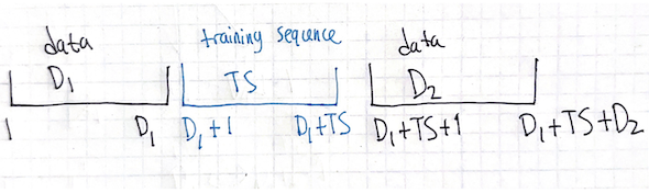
We note that all the lengths are correct:

• First data section is from \(1\) to \(D_1\) so its length is \(D_1-1+1 = D_1\)
• Midamble is from \(D_1+1\) to \(D_1 + TS\) so its length is \(D_1+TS-(D_1+1)+1 = TS-1+1 = TS\)
• Second data section is from \(D_1+TS+1\) to \(D_1+TS+D_2\) so its length is \(D_1 + TS + D_2 - (D_1 + TS + 1) + 1 = D_1-D_1 + TS - TS + D_2 - 1 + 1 = D_2\).
• Total burst is from \(1\) to \(D_1+TS+D_2\) so its length is \(D_1 + TS + D_2 - 1 + 1 = D_1 + TS + D_2\).

It’s clear how we can isolate any particular section of this burst before it has passed through a dispersive channel.

notation review for intervals of integers #

• \([1,5]\) means “1 to 5, inclusive of the bounds (”closed”) on both sides”, and represents \({1,2,3,4,5}\)
• \((1,5)\) means “1 to 5, non-inclusive of the bounds (”open”) on both sides”, and represents \({2,3,4}\)
• We also can have left-closed right-open: \([1,5)\) is inclusive of the \(1\) but not of the \(5\) so we have: \({1,2,3,4}\)
• And likewise with left-open right-closed: \((1,5]\) represents \({2,3,4,5}\)

adding² channel effects #

As the subtitle in the header insinuates, a dispersive channel is represented by a convolution. The structure of convolution tells us that each transmitted sample will affect multiple received samples, and the channel vector’s finite length tells us it’s not gonna be all of them.

We note that a single sample will be “smeared out” by a channel of length \(L\) onto a span that’s \(L\) long:

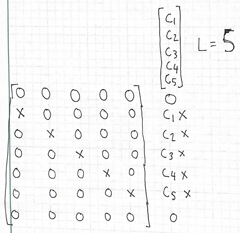
As for the indices, if this sample lives at index \(n\), the index of this little “span of influence” will be \([n, n+L-1]\). Why these indices?

• the starting index: We currently don’t care³ about absolute delays, just what happens inside the delay spread. Remember the “ideal coaxial cable” thought experiment from our last post: the problem remains identical no matter how much ideal coaxial cable lives between our receiver antenna and our receiver frontend. We can therefore say that the input sample at index \(n\) gets transmogrified by an “identity channel” (impulse response of \([1]\), it doesn’t change the signal at all) to be an output sample at index \(n\) – no need to add any offset.

• This means that the first output sample to be affected by our input sample will be at index \(n\), which justifies the left-closed (includes its boundary): \([n,\)

• the ending index: If the “span of influence” is \(L\) long, the last sample that is affected by our input sample will be at index \(n+L-1\). This justifies the right-closed (includes the boundary): \(,n+L-1]\)

Going back to our “single element convolution” example, if the \(x\) input sample lives at index \(10\), the first nonzero output sample lives at index \(10\) by fiat. We observe nonzero output samples at \(11, 12, 13, 14\) as well. Output sample \(15\) and beyond are zero, as are samples \(9\) and lower. This means that we have nonzero output at \([10, 14]\), and if we let \(n=10\) and \(L=5\) we get \([10, 10+5-1]=[10,14]\), which matches up with what we see.

how the burst structure gets preserved by the convolution #

There is a definite structure to the transmitted burst: known data (the training sequence) sandwiched by unknown data. In realistic systems, the designers will select a training sequence length longer than any reasonable channel they expect to contend with, and so we expect:

• some received samples will be a function only of unknown data
• some received samples will be a function of unknown data and training sequence bits
• some received samples will be a function only of training sequence bits

To figure out which received samples are which, let’s draw out what happens when our burst gets convolved with a channel of length \(L\). Each transmitted symbol will get “smeared out” onto an \(L\)-long span, and we focus on the symbols at the boundaries of each section.

The center line represents what the receiver hears, and for clarity, we draw the unknown data sections above the center line and the training sequence below the center line.

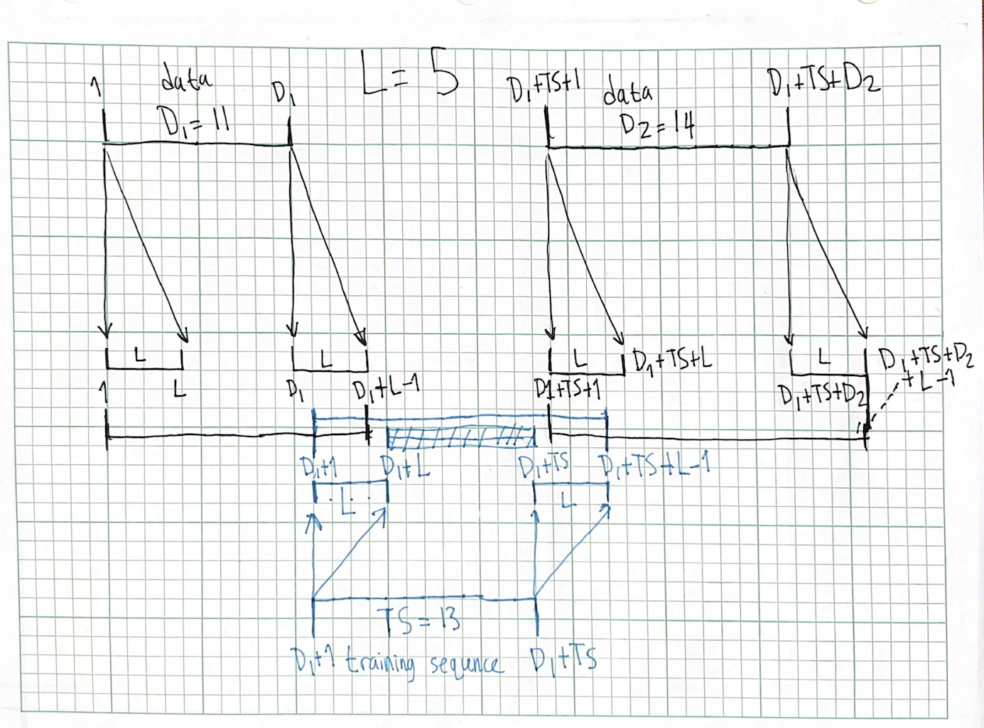
Things are much more clear now!

• \([1, D_1]\), with length \((D_1)-(1)+1=D_1\): the output’s only affected by the first data section
• \([D_1+1, D_1+L-1]\) with length \((D_1+L-1)-(D_1+1)+1=L-1\): the output is affected by the first data section and the training sequence
• \([D_1+L, D_1+TS\) with length \((D_1+TS)-(D_1+L)+1=D_1+TS-D_1-L+1=TS-L+1\): the output is only affected by the training sequence. This is the section we use for a least-squares channel estimate!
• [\(D_1+TS+1, D_1+TS+L-1]\) with length \((D_1+TS+L-1) - (D_1+TS+1) + 1= D_1 + TS +L -1 -D_1 -TS -1 +1= L-1\): the output is affected by the training sequence and the second data section
• \([D_1+TS+L, D_1+TS+D_2+L-1]\) with length \((D_1+TS+D_2+L-1) - (D_1+TS+L) + 1= D_1 +TS + D_2+L - 1 -D_1 -TS -L +1 = D_2\). This part is only affected by the second data section.

Now let’s sum⁴ up all those lengths to see if our work checks out: \((D_1) + (L-1) + (TS-L+1) + (L-1) + (D_2) = D_1 + L -1 +TS -L +1 +L -1 +D_2 = D_1 +D_2 +TS +L -1\). This is indeed what we get when we convolve a vector with length \(D_1+D_2+TS\) (the total length of the burst as it’s transmitted) by a vector with length \(L\) (the channel)!

As usual, if you notice an error in my work, I’d be very grateful if you could point it out to me.