GSM receiver blocks: rough notes on coarse timing estimation

In this GSMish scenario we don’t actually need pinpoint/“fine” timing/phase accuracy, since a good enough Viterbi demodulator effectively “cleans up” remaining timing/phase offset as long as it’s fed with an accurate enough channel estimate (especially if it’s able to update its channel estimate).

small timing offsets don’t matter too much for this demodulator #

In a simplistic scenario, if our channel looks like \([1,1]\), it doesn’t matter if the channel estimator outputs \([1,1,0,0,0,0,0,0]\) or \([0,1,1,0,0,0,0,0]\) (here we are using the classic GSM design choice of making our channel estimator handle channels of length 8) or anything up to \([0,0,0,0,0,0,1,1]\) – we get the same results at the end. If we’re misaligned enough to get \([0,0,0,0,0,0,0,1]\) we are leaving half the energy in the received signal on the table, so we do want as much energy possible in the actual channel’s impulse response to appear within the channel estimate the demodulator is given.

Of course, with a more realistic case, the actual channel won’t be just two symbols long, this is terrestrial radio, not a PCB trace / transmission line nor an airplane-to-satellite radio channel :p

coarse timing offsets matter a lot to the channel estimator #

In the case where the physical channel has a length commensurate with the channel length designed in the channel estimator / demodulator, we want to make sure that our least-squares channel estimator gets aimed at the right place in the burst – if it ingests lots of signal affected by unknown data (as opposed to known training sequence data affected by an unknown channel), its output will be kinda garbage.

form is emptiness, cross-correlation is matched filtering #

We’d be at an impasse¹ if the least squares estimator was our only tool here, but we have a simpler tool that’s more forgiving of misalignments: cross-correlating the received signal against the modulated training sequence. Another way of thinking of this is that we’re running our received signal through a matched filter (with the reference/template signal the modulated training sequence) – it’s literally the same convolution.

Doing this gives us something that looks like this:

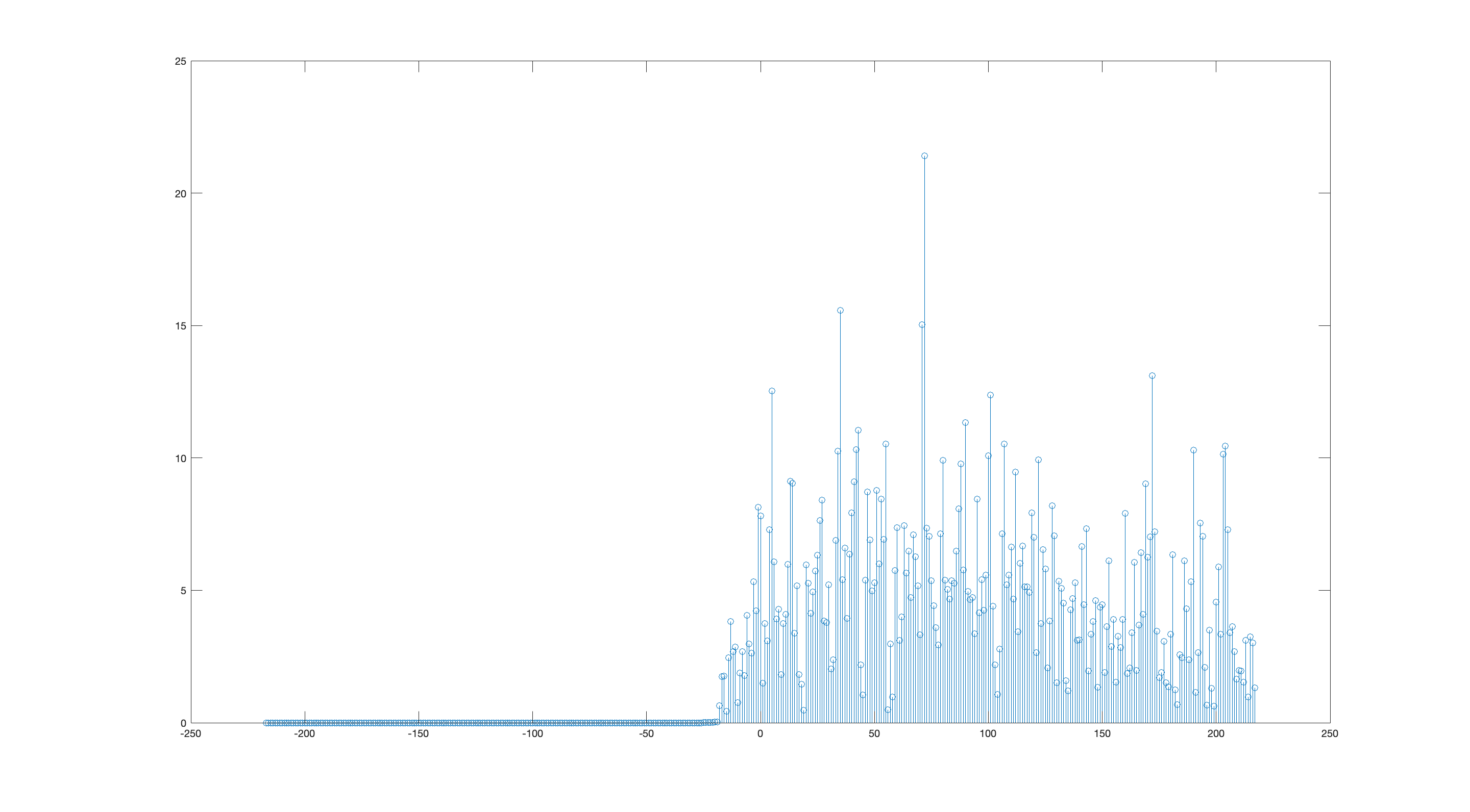
Using the Mk I eyeball, it’s pretty clear where the training sequence lives – at the tallest peak.

For implementation in software or gateware, we can encode this logic pretty easily: calculate the correlation, then iterate and look for the biggest peak. However, we notice that there’s a bunch of spurious peaks all around, and it’d be quite bad if we accidentally matched on a spurious peak: the channel estimate would be garbage, and the output of the demodulator would be beyond useless, since it wouldn’t even be starting off at the right spot in the signal.

We can avoid this failure case by running the correlation on a smaller window, which reduces the chances of hitting a false correlation peak. We determine the position of the smaller window using our prior knowledge of the transmitted signal structure – where the training sequence lives relative to the start of the signal – and an estimator to determine when the start of the signal happens.

It’s pretty easy to determine when the start of the signal happens: square/sum each incoming I/Q pair to get a magnitude, and keep a little window of those magnitudes and when their sum exceeds a threshold, well, that’s when the signal started.

We use this to narrow down the possible locations for the training sequence in the received signal. However, we still should run the correlation since this energy-detection start-of-signal estimator has more variance than the correlation-based timing offset estimator.

why training sequences are like that #

Incidentally, the GSM training sequences (and lots of training sequences in other well-designed wireless communications systems) have interesting properties:

• their power spectra are approximately flat
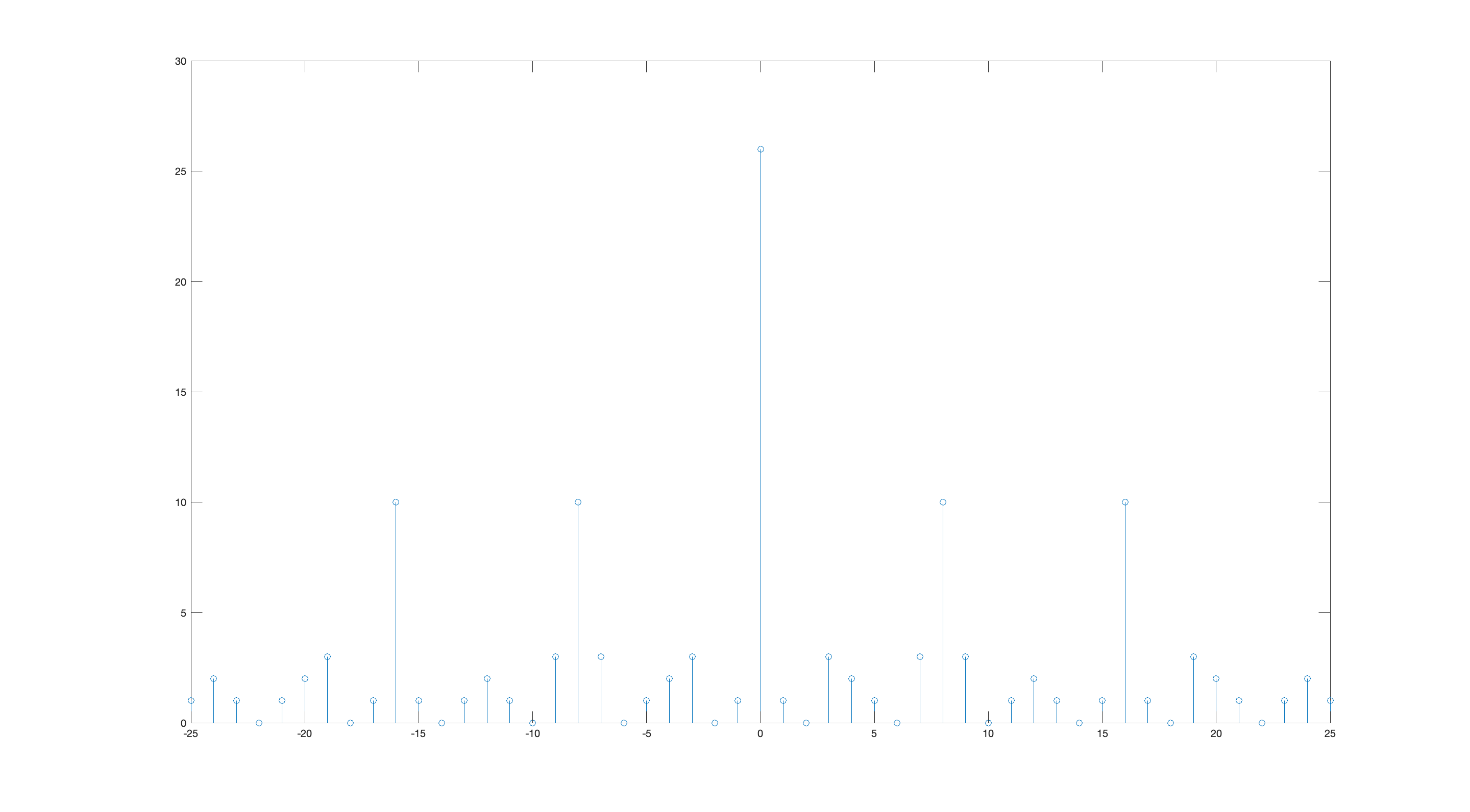
• their autocorrelation have a tall narrow peak that approximates an impulse, and has much less energy elsewhere

The former is a desired property since we want to evenly probe the frequency response of the bandpass channel. Spreading the training sequence’s power unevenly (lots of power in one part of the passband and much less in another part of the passband) causes a worse signal-to-noise² ratio in the parts of the passband with less training sequence power. It’s a zero-sum affair since the transmitter has finite transmit power.

The autocorrelation property not only lets us use these training sequences for time synchronization, but it lets us use correlation as a rough channel impulse response estimate. If we’re satisfied with a very suboptimal receiver, we can just use the correlation as our channel estimate. However, least-squares generally will give us a more accurate channel impulse response, since the autocorrelation of the training sequence is not 1 at zero lag and 0 elsewhere – there’s little sidelobes:

truck-correlation (it’s like auto-correlation but with 18 wheels) #

If you don’t have a good intuition for what a narrow autocorrelation does here, you can develop one by going to a loading dock or a construction site and paying attention when big trucks or earthmoving equipment back up. See, those big rigs are required to have a back-up beeper to warn bystanders that the driver is backing up and can’t see well what’s behind the vehicle.

pure tone: easy to detect, hard to localize #

There’s two common types of back-up beeper, and unfortunately the more common kind outputs a series of beeps of a single pure tone (without changing frequency between beeps). If you close your eyes and only use that sound to determine where the truck is, you’ll find it’s quite a difficult task: it seems like the sound is coming from everywhere! The brain has a variety of mechanisms to localize sources of sound, and besides the ultra-basic “find which ear is receiving the loudest signal” method many of them kinda boil down to doing cross-correlations of variously-delayed versions of the left ear’s signal against variously-delayed versions of the right ear’s signal, and looking for correlation peaks. Seems familiar!

Unfortunately, the pure sine tone is the worst possible signal for this, since there’ll be tons of correlation peaks (each oscillation of the sine wave is identical to its precursor and successor), and if there’s audio-reflective surfaces around you and the truck, there’ll be tons of echoes too. Ambiguities galore! More spurs than a cowboy convention!

Ironically, the most useful (for angle-of-arrival localization) part of the pure-tone truck beeper’s signal is the moment the beep starts³, since the precursor is zero – the rest of the beep is comparatively useless for localization (an estimation task) but extremely useful for knowing that there’s indeed a truck somewhere in the neighborhood backing up (a detection task). The start and end of the beep are the most spectrally rich part of the beeper’s output, and this is indeed what we expect.

The pure sine wave is the easiest possible signal to detect (with our friend the matched filter), but the worst possible signal for localization; and this irony is why you can hear truck back-up beepers from uselessly far away but can’t easily tell which truck is backing up.

white noise: hard to detect, easy to localize #

Fortunately, there’s truck back-up beepers that output sounds far more amenable to localization: little bursts of white noise. If you haven’t heard those, you can find a youtube video of those in action, play it on your computer, and try and localize your computer’s speakers with your eyes closed.

You’ll notice that this is basically the optimal signal if you want to do angle-of-arrival estimation with delays and correlations – there’s only one correlation peak, and it’s exactly where you want it. It’s also extremely spectrally rich, and it has to be, since spectrally poor signals have worse autocorrelation properties. It also has the advantage of “blending in” with other noise: on-and-off bursts of white noise get “covered up” by white noise (and become indistinguishable from white noise) very quickly, a pure tone is much more difficult to cover up with white noise.

This is what a good training sequence looks like: simple correlation gets you a passable estimate for the channel impulse response along with the timing offset, since the autocorrelation approximates an impulse. Also, the spectral richness ensures that all the frequency response of the bandpass channel is probed.

A Viterbi-style demodulator is a controlled combinatorial explosion #

I don’t think there’s too much useful we can do with the coarse correlation-based channel estimation to enable a more accurate channel estimation with more advanced (least-squares) methods – I had imagined looking at the coarse correlation-based channel estimate and looking for a window with the most energy and then doing a least-squares channel estimate only on that window, but I don’t think that actually has realistic benefits.

However, that idea (focusing on where energy is concentrated in the channel impulse response) does point to a more fructuous⁴ game we can play with channel impulse response: transforming the channel to squash the channel’s energy as much as possible into the earlier channel coefficients, and this is called “channel shortening”. Channel shortening is interesting because rather than having to delay decisions until the last possible moment, we can commit to decisions earlier, which reduces the computational burden (and area/power requirements) on a Viterbi-style demodulator pretty significantly.

If the impulse of the channel is highly front-loaded into, say, the first 3 symbols, we force a decision after only 3 symbol periods, since the likelihood of something after that making us change our mind is very unlikely. We still keep track of the effect of our decisions for as long as the channel lasts, since otherwise we’ll be introducing actual error (even if we make all the right decisions) that’d be pretty harmless to avoid: once we made the decisions, figuring out their effect is as simple as feeding them through a channel-length FIR filter.